| Previous Page | Contents | Next Page |
Before you start to reduce a set of runs with Qed, it would be wise to establish a pattern of directories to make life easier. I make a new directory, usually named after a WET run, or the target object, with a set of subdirectories to keep things orderly. Of course, this is MSDOS, not Unix, so we must use the '\' character as a pathname separator, which can get printed following the name of a directory to tell you it's not a regular file. I struggled through many versions of MSDOS trying to get them to use '/' like Unix does, but Microsoft ultimately defeated me. Curiously, Internet Explorer understands pathnames with '/' in them, but the rest of Windows/MSDOS does not.
My working directory looks like this to start with:
\xcov99\
Raw data are first copied into the raw\ directory, and any accompanying observer's log files into log\. Two simple batch files that know about this directory arrangement can keep you from having to type the same thing over and over again. (I put 'z' in front of names so they will show up at then end of a file listing, where I can see them easily). The command zget filename will find the file in the raw\ directory (if it's there), copy it to the working directory making sure the line endings are MSDOS-like, and start up Qed to process it. When you finish reducing the data, write the output and quit the Qed program, the command zput filename will move the finished data files into the red\ directory, assemble the raw data file and the opfile into an arq file and store it in the directory arq\, and move the opfile itself into the opfiles\ directory. If you wrote more than one .op file, zput uses the latest one it can find. During the reduction process, you can suspend Qed (the F6 key does that) and consult any log files in the log\ directory if you need to.
This directory setup works well if you are reducing (or re-reducing) WET run data. The command
qmrg red\*.1c*
will assemble all the reduced data for channel 1 into a single light curve, averaging runs together wherever they overlap in time. Qmrg will complain if you try to make a single light curve out of data for different targets. Should you have some misgivings about a single run, after you see it in context with its WET companions, you can use the command
qed arq\filename.arq
to run Qed on it again. If you did all your marking first, before any other operations (highly recommended), then the startup Run mode screen will show you the data already marked, with the reduction commands present but not yet executed. If additional marking (or unmarking) is needed, do that first. It is then easy to step through the unexecuted commands, changing parameters or adding additional operations, as needed to improve things.
If you want to reduce the whole data set a second time, the command
for %a in (arq\*.1*) do qed -b %a
will re-reduce all the channel 1 data in the WET run, using the recorded lists of operations attached to the raw data files. (If you ever need to put this command into a batch file, change %a to %%a in two places.)
Let's reduce another run, this time taken with the Texas 3 channel photometer, from a later WET run but with the same target star (PG1159). The run (jlp-0145) is in native Quilt format, but Qed can also read SAAO native format, and (with qform.exe available) French format data taken with the Chevreton photmeter. Once running, it can also read and write Dred .flg format data, if you ever need to do that. You can also read in a run with Qed already running: the F7 key (either in Set mode or in Run mode) prompts for an input filename and reads it in (if it can). The last filename entered is repeated after the prompt, and can be edited to remove, say, a typo. We first encounter the Set mode window, so let's examine that to see what we have.
On startup, Qed does a lot of checking, and if all you see is the friendly notation at the bottom all is well. If it can't find everything it needs, it will tell you about it, perhaps displaying several messages one after another on the bottom two display lines, giving you time to read each one before replacing it with the next one. It is wise to heed them, and to fix whatever Qed is complaining about before you proceed. If it can't identify the photometer, for example, perhaps because the observer didn't use a notation Qed understands, try to find out what is normally used (consult the qed.tbl file) and then edit the header for the run to keep Qed happy, or add the new name for the photometer in addition to the ones already present in the qed.tbl file. The Q9 data, and the stuff in qed.tbl are all normal ASCII text so any text editor should work.
Data from Q9 (or translated to this format, if from some other program), show up in their boxes in the Set mode window when Qed first comes alive. Entries can be edited if need be, and will overwrite the original entries for subsequent operations. Qed consults all of the Set mode window entries except for the Telscp and Progrm lines, so errors in any of the others can cause errors in the output from Qed. For example, the Where line establishes the longitude and latitude for the observatory, the Photom line is used to decide on the default deadtime corrections, etc. The Drive line selects the drive ('C' by default) on which Qed writes the output data. If you need to, you can change this output drive to, say, 'B' and then, after using the subst command in MSDOS to define 'B' to be whatever directory you choose, find the output data written there. I usually leave it alone so the data get written to my working directory, where the zput command can find them and squirrel them away properly.
When you edit a line in Set mode, whatever you type in will be checked for legality whenever you move the cursor off the edited line. No news is good news: Qed, like Q9, is silent unless it takes offense at what you entered.
The Texas 2 and 3 channel photometers have filter wheels which are motor-driven, and the integration times for each filter are shown in the window, in seconds. By convention, an entry only in the first filter line, with 0.000 in the other three, means the motor was not active during the run, and the filters were not moved. More than one non-zero entry indicates that filter motion took place. You can't edit these integration times in Qed because that would really mess up the reduction process. Filter motion takes some time, and the F2 key invokes a sub-window showing the actual integration time and the time it took for the filter to get moved to the next position. This information was resident in the original Q9 header, but only shows up if you ask about it. The filter changing time plus the actual integration time will always add up to the time chosen by the observer: filter changing time is deducted from the time entered, so the total time per measurement stays constant at the time requested. A sub-window brought up by the F3 key shows the filter starting position for each channel, and the Motor line entry indicates which (if any) motors were turned on during the run. This entry is irrelevant when only a single filter was in use, as in this case.
Qed is rarely (if ever) used to reduce multicolor data, and is internally quite complicated because it has the ability to do so. This, it turns out, was a poor design decision, and any subsequent rewrite of Qed should probably just deal with one filter. The original multicolor data can be unlaced into separate files and dealt with one at a time.
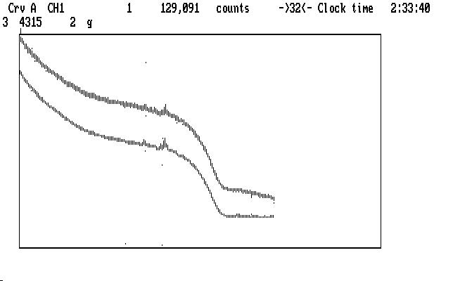
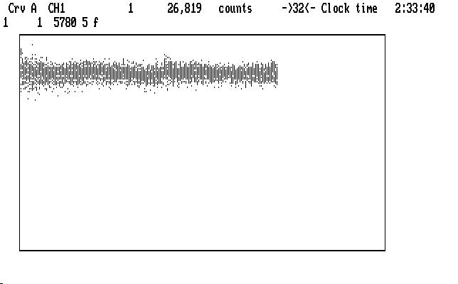
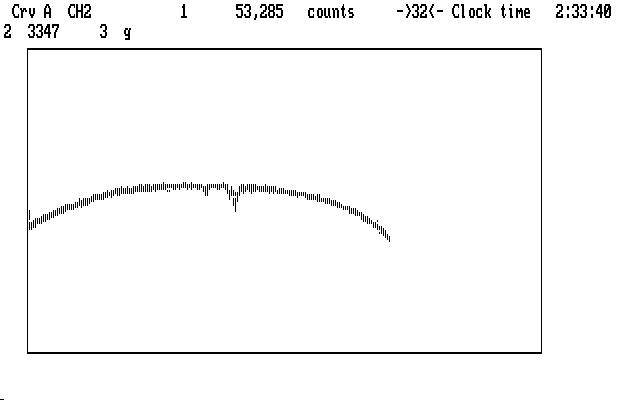
The initial Run mode display doesn't look much like our previous example:
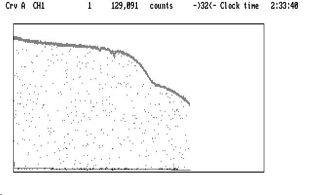
| Fig. J01 |
Ch2 is topmost and, in addition to its funny shape, splatters points below the curve pretty much everywhere. These are interruptions for guiding, which in this case are quite frequent. The funny shape we will understand in a moment. We notice that Qed had to compress the run by 32, instead of 16 in the first example, to get it all on the screen at once; that's because this run used 5 second integrations for each data point, while the earlier one used 10. Same star, though.
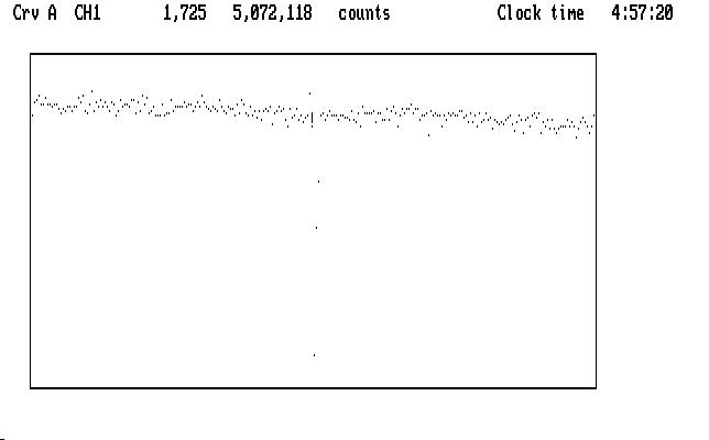
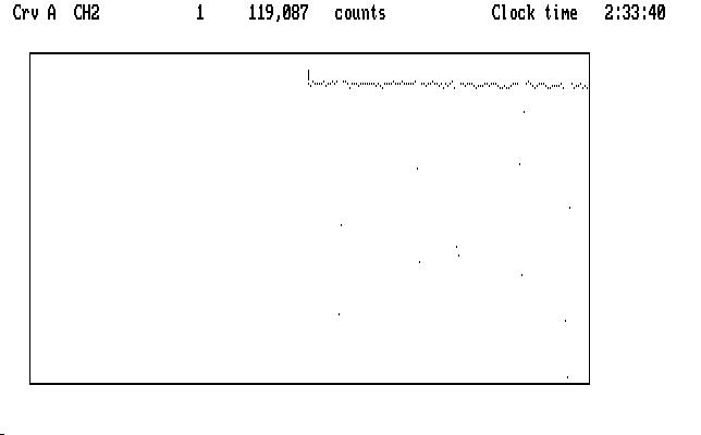
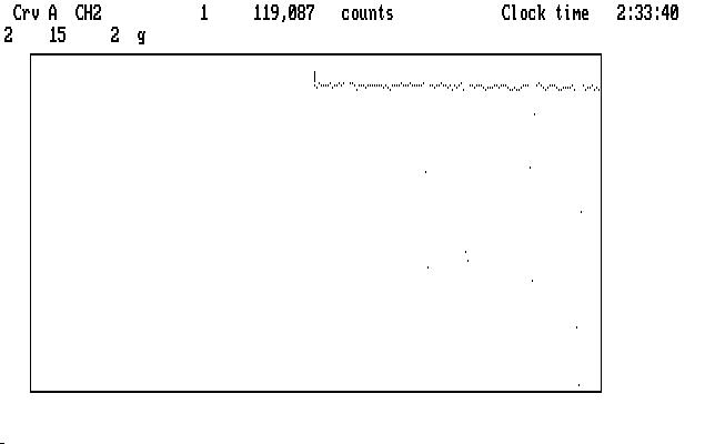
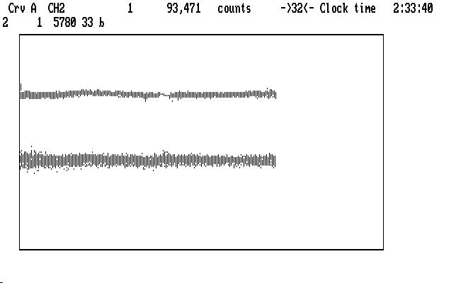
Ch1 is mashed along the bottom of the display. Remember Qed autoscales in both X and Y on startup, so we might guess that there are some very high data points in Ch1. If we suppress Ch2 we can see them clearly:
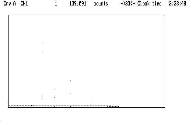
| Fig. J02 |
We must deal with them first, because they are a hazard. The next image shows what we see in the uncompressed curve, with the cursor marking one of the very high points:
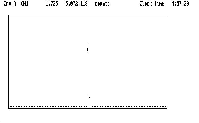
| Fig. J03 |
If we magnify the display in Y (using PgUp) without moving the cursor we notice that the bad data point appears to fall right in with the good points in the light curve:
| Fig. J04 |
The display wraps around in Y, so points that get magnified off the top reappear at the bottom, and can look like they are a part of the normal light curve when they are not. We avoid this ambiguity completely if we mark the very high points first, before we magnify the curve in Y to see the rest of it.
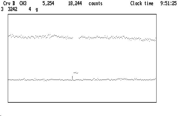
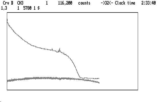
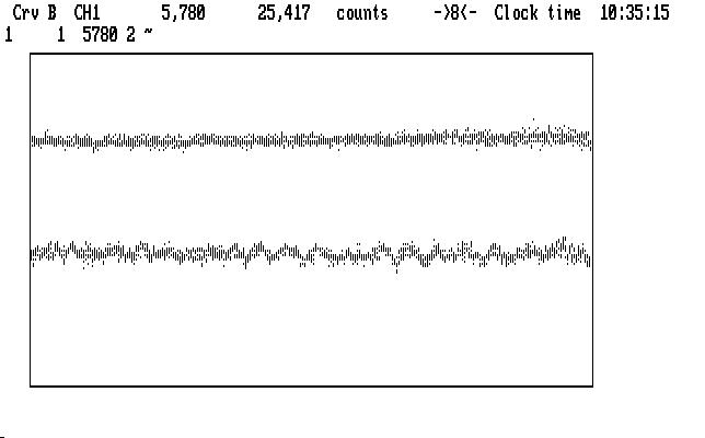
This is a 3 channel run, so we have sky data in channel 3 to deal with. If we make it visible using Alt-3, so it replaces the Ch2 data in Crv B, we find it looks very much like the data in Ch1: all mashed down due to very high data points. We also must mark those first, before we magnify. We can then magnify both Crv A and Crv B together to see this, with Ch1 on top and Ch3 sky below it:
| Fig. J05 |
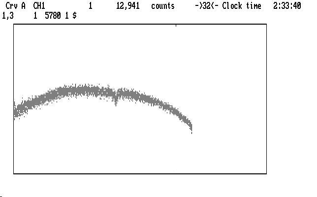
There are still a few wayward points, which we can now mark with 'g'. If we examine the Ch1 curve (or consult the log file for this run) we find that there is a typical sky measurement near its end, where the curve is low and nearly flat. As before, we mark it with 's' (and it blinks in appreciation). Remember that the sky data in Ch3 are taken with a detector that has a sensitivity different from the Ch1 detector (and the Ch2 detector, too) and we calibrate those differences by measuring sky with all 3 at the same time, at least once during a run. Qed understands this convention; if there is more than one such sky reading, they are averaged together to get the correction factors. The next image shows an expanded view of this region after we have marked the sky points, and have put the cursor on Ch3:
| Fig. J06 |
and the next shows the compressed view, with the Ch1 sky showing up as a single dot because of pixel stacking:

| Fig. J07 |
Qed doesn't require that we reduce both channels together the way we did in our first (2 channel) example, so let's reduce just Ch1 to see how it goes. In this case we use the lower case version of the commands, and we'll step through them one at a time. Our first command is 'd' (or D; they do the same thing) to correct for the dead time in all 3 channels. It doesn't have much of an effect on the light curves, because the correction is small at the counting rates encountered here. It can matter a lot if the counting rates are high. Qed will use the default values it knows about for a particular instrument, but you can override them by entering deadtime parameters (in ns) in front of the 'd' command. The first parameter typed in will be applied to Ch1, then next to Ch2, and the third to Ch3. Use the Enter key to separate them.
Our verbosity level is set at the default (1) so we get only warning and error messages displayed, but we can make Qed temporarily gabbier by preceding any command with 'v'. If we do that, then after the 't' command we get this display:
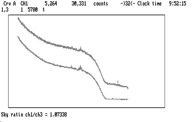
| Fig. J08 |
with the detector sensitivity ratio displayed. It looks OK; the Ch1 and Ch3 detectors are usually chosen so their sensitivities match fairly well. At this point the ratio has been calculated, but not yet applied, allowing us the option of typing in a different one before the 'p' command, which corrects the sky measurements by multiplying by this ratio. Any value you enter from the keyboard will take precedence over other possible ratios. If Qed does not find a sky measurement to use in this calculation (perhaps because we marked the sky measurement in Ch1 with 'g'), it will examine its copy of the history file (from qed.his) and if it can find an entry corresponding to this instrument (PG Mudgee) it will use that, and warn you it is doing so. If it can't do that, Qed will use the default ratio taken from the qed.tbl file for this instrument.
Our next step is to prepare the sky for subtraction using the 'p' command. Since this is a 3-channel run, the first 't' command we execute copies the sky from Ch3 into buffer 4, so we will have an original copy to use on the other channel later. The 'p' command multiplies the Ch3 sky data by the correction ratio found by the 't' command.
We are ready to subtract sky now. Before we do that, though, we may want to smooth the sky data to minimize the amount of noise we introduce into the Ch1 light curve. We notice that there are a couple of places in the run where both channels brightened up for a short time. This is typical of moonlit clouds passing near, or over, the target object; moonlight gets scattered into the photometer aperture. We can hope that the same amount was scattered into Ch3 as into Ch1, so it will come out nicely when we subtract the sky. If we smooth too much, however, it won't.
Here is a place where we can use the Qed handy-dandy backup process to try things. Try smoothing Ch3 (the '~') command preceeding it with different values, then subtract the sky ('Alt-S') and see what happens. Too much smoothing will leave a lump in the Ch1 curve, too little will add noise everywhere in Ch1. You can then back up (Ctrl-B twice) and try a different value. (This is Art. You expected Science?) In this case, a smoothing coefficient of 9 is a reasonable compromise, yielding the result shown below, with Ch1 nearer the bottom:
| Fig. J09 |
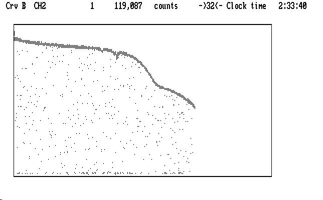
Note that the really funny shape of the light curve has been much improved. As you may have guessed, there was a lot of moonlight during this run, and moonset happened before the run finished. If you didn't know what moonset looks like photometrically, the image above shows it to you.
If we suppress Ch3 and then magnify with PgUp, we get the curve shown in the next image:
| Fig. J10 |
and we notice the notch where the lump used to be. Different amounts of smoothing don't really help here; some light has been lost from a thin cloud passing over the target. We are not out of tricks, however. The next image shows a (somewhat) uncompressed view of the notch, with a range set to span it:
| Fig. J11 |
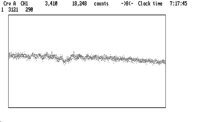
The leftmost cursor mark is blinking. We will invoke the polynomial fitting process, in which a polynomial is fitted to the selected region of the light curve, and then that region (only) is divided by the fitted function. Qed supports polynomials with orders from 1 to 5. In this case we eyeball the notch and decide a cubic fit (order 3) is the lowest we can use to do the job. (You can try other orders, and other spans, backing up and trying again until you are either happy with it, or too tired to care.) The next image shows the result of using the command '3f' over this range (290 data points, starting at 3121, as shown in the 2nd display line):

| Fig. J12 |
The remaining curvature is typical of a long run with changing amounts of atmospheric extinction, which we can calculate (based on the location of the observatory, the time of day, and the location of the target object in the sky) and then correct the curve. All we know how to calculate is the effect of atmospheric scattering and absorption, and both depend on the color of the light from the target star, so the amount of the correction changes from one star to another (from the Ch1 star, say, to the Ch2 star). We adjust the coefficient we give to the extinction routine in a (usually futile) attempt to take this into account. Again, trial and backup can help here, to some extent. Remember, though, that the real atmosphere has a lot of small, often opaque aerosols that we try to look though, and these can vary a lot from one part of the sky to another. We make no attempt to model that stuff because we don't know how.
Smiling cheerfully, we use the command '0.35e' to get this result:
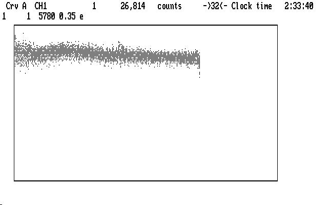
| Fig. J13 |
which actually doesn't look too bad. The curve is everywhere higher than before the correction, since the extinction model tries to remove all of the extinction effects, including the air straight overhead. There are a few small lumps and bumps still showing, and if we are really offended by them we can apply the 'f' command to the whole light curve and try to make it better. This may not really be necessary, but if we do it, we get this result:
| Fig. J14 |
Our next job is to reduce the Ch2 data. We can proceed from here in two ways: marking at this point in the reduction process, or backing up so the marking in Ch2 is contiguous with the marking we did in Ch1. The second option is somewhat better, since replay is much simpler if you do this. The command 'Alt-Shift-B' will undo all of the reduction commands (but not the marking operations) and doesn't erase them; they are still there, but now not executed. The F5 keystroke will display the last of the encoded operations like this:
1  3572     1  g
1  5779     1  g
1  5255     1  g
1  5264     1  g
3  2389     4  g
3  2853     4  g
3  3242     4  g
1  5256     8  s
*-->
1     1  5780 15 D
2     1  5780 15 D
3     1  5780 15 D
1,3     1  5780  t
1,3     1  5780 1.0734 p
3     1  5780 9 ~
1,3     1  5780 1 $
1  3124   289 3 f
; long -104.02167 lat  30.67167 ra  12.02368 dec  -3.72244 dtt 59.184
1     1  5780 0.35 e
1     1  5780 5 f
where the funny arrow is just above the next command ready for execution. Note the encoded marking for Ch1 and Ch3 and then, at the end, the sky marking for Ch1. If we now mark the Ch2 data, the operations will go above the *--> mark. Note that Qed put in a kind of comment line just before the 'e' command, giving the values it used in the extinction calculation, so replay can use the same values. Qed tries to do the Right Thing, quietly.
Now for channel 2. We can use Shift-2 to put Ch2 data into Crv A, and note the discouraging number of bad points we have to mark (remember our first look at this run, Fig. J01). Do we really need to do this? (Answer: yes. If you want life to be easy, you have chosen the wrong profession.) Be of good cheer: many modern-day runs use autoguiding, or remote guiding, so the number of bad points is vastly reduced. For this run, though, we will use the 'm,M' commands (mnemonic: magic) to make things go faster. The next image shows the curve ready to start marking, after executing the 'Tab' and 'x' commands:
| Fig. J15 |
For these commands to work properly, we must tell Qed that the cursor is sitting to the left of a "good" region of the light curve. In this case the start of the curve is as good as any other part, except that there are a couple of bad points nearby (for this operation, Qed examines the first 20 unmarked data points to get things going) so we must mark them with 'g', then return the cursor to the start of the light curve. The next image shows the curve after we do this:
| Fig. J16 |
Now the 'm' command will set up the algorithm to find deviate data points, starting at the cursor location, and the 'M' command will make them blink. The 'x' command will compress things so you can see how well the deviate identification has been done, after clicking on the link:
| Fig. J17 |
It's not perfect, but it's pretty good. In theory, all of the guiding points will blink and none of the light curve will blink. If this ideal is not achieved you can try giving the 'M' command a parameter. The default value is 10, and a smaller value will make the process less sensitive, and a larger value will make it more sensitive. A different location for the cursor prior to the 'm' command might help. You can start all over again by using the the 'U' command to stop all the deviates from blinking. If the magic works over the first part of the light curve but fails later, you can apply the algorithm to the later part of the light curve by moving the cursor there, and using 'm' and then 'Ctrl-M', which only looks for deviate points downstream of the cursor.
Assuming we can get it to work (it works fine on this run using the start of the curve and the default value for 'M'), we can now proceed to mark the bad points, using the 'n' key (for "next") to jump to the next deviate point, which is much faster and easier than moving the light curve with the '<-' key, as we did before. With one finger on the 'g' key and another on the 'n' key, you can jump along at a good rate. The 'l' key jumps the other way, to the last marked or deviate point, in case you missed one. If a blinking deviate appears to be part of the light curve and not really a deviate at all, the space bar restores it to normal. The space bar activates a general "unmark" action for any one point, or a chosen range of points.
After we have marked Ch2, including its sky measurement, we can replay the Ch1 reduction with the command 'Alt-A', and then step through the Ch2 reduction (remember the 'D' command is already done) with the 't', 'p', and 'Alt-S' commands. The next image shows what the curve looks like after sky subtraction:
| Fig. J18 |
We can remove the smaller bump using the range-limited polynomial fit as we did on Ch1, but the second is just too large and messy to keep. We'll just mark it as garbage, and bridge over it like any other data gap. This is OK for Ch2 since we don't plan to analyze it in detail later, but would not do for the target data in Ch1. We'd have to chop the run into two parts (by using '|' instead of 'g' to mark the bad data region). Physically, on the photometer, Ch1 and Ch3 (the sky channel) are very close together, and look at immediately adjacent parts of the sky. That's why the passing cloud had such similar effects on them. Ch2, however, looks at a part of the sky some distance away (where a monitor star was found, in fact) and was affected somewhat differently by the moonlit cloud. This explanation doesn't improve the data any, but it lets us feel a bit better about it.
We execute the 'e' command on Ch2, and remove an upward slope with 'f', then redisplay the reduced Ch1 data in Crv B. After bridging both curves, the bridges blink, and we have the result shown below:
| Fig. J19 |
This is a considerable improvement over the run we started with. We can now write everything to disk with the F9 command.
If you worry that the pulsations we are looking for don't show clearly in Ch1, be assured they are there, although somewhat the worse for noise. The shorter integration time, the scattered moonlight and a smaller telescope conspired to add a lot of noise to the measurement, compared with our earlier example. We can, at least, approximate what a longer integration time might look like if we smooth Ch1 with the command '2~'. The last part of the run, where the moonlight is least, expanded to the equivalent in our first example, is shown here, with Ch2 on top:
| Fig. J20 |
Our work has not been in vain.
| Previous Page | Contents | Next Page |