BRIDGING: TO 'b' OR NOT TO 'b'

The main purpose of data reduction is to remove instrumental artifacts from the data set so we can analyze the result with some confidence. If we fail to remove them completely, or if we introduce other artifacts during the reduction process, we may interpret an artifact astrophysically. There are an embarrassingly large number of published observational papers which do exactly that. I have a little list.

The bridging process in Qed evolved primarily from the need to interpolate between isolated sky readings in 2-channel data, so it includes extrapolation at the ends of the light curve as well, in case the observer(s) didn't start and end with sky. They're supposed to, of course, but it would be churlish of Qed to refuse data not taken exactly as specified. In an attempt to minimize the effects of noise, the 'b' command accepts a parameter, indicating how many data points on each side of a data gap should be averaged together to anchor the bridge. The process then draws a straight line between the two averages, replacing the 'g'-marked data points but leaving the other data points alone. With a bit of experimenting and backing up, it's usually possible to find a value that does a good job on the whole light curve. The 'b' command can be limited to a range, if you choose, so you can use different parameters on different parts of the light curve, but I've never found I really needed to do that.

Extrapolation often doesn't work very well. In this case two contiguous regions near the end of the light curve are averaged together, then a straight line is drawn between them and extended beyond the end of the unmarked data. If it really does terrible things, you can poke in an artificial data point (Alt-P) in the proper place to constrain it, thus forcing the bridging algorithm to interpolate.

So isn't the process of bridging across data gaps actually modifying the data in a way the star would never have done? Yes. So why do we do it? Because leaving a gap introduces an artifact in the final result that may be far worse than a bridge. Stars don't quit sending light when we're not recording their data, and our analytical tools all assume we have data that are contiguous in time, and that goes to infinity in both directions. If we have a gap in the data, the Fourier transform process that we use to identify periodic frequencies in the light curve will introduce spurious frequencies due entirely to the data gap. We call them "aliases", and we try to identify and discount them in our analysis. If the gap is very short compared with the periods really present in the star, then the alias it introduces will appear primarily (but not exclusively) at very high frequencies. If the gap is longer the alias will appear at somewhat lower frequencies, and if the gap spans several cycles of the star's real period then the alias can easily be confused with a real stellar pulsation period.

Here's an example of how the bridging process works, an uncompressed segment of the first run we reduced Tol-0011. Ch1 is on top, Ch2 below, with the stellar pulsations clearly visible in Ch1.

Fig. T14

The bridge in Ch1 spans the place where sky was measured, with a corresponding place in Ch2. The earlier bridge in Ch2 spans the region where instrument alignment took place, as we saw in Fig. T10.

We can (and do) adopt a rule of thumb: if the gap is significantly shorter than the shortest known period in the star, then bridging the gap is kosher. If the gap spans several periods, then it probably isn't, because we have then lost the information we seek, and replacing real periodic wiggles with a flat bridge does damage to the light curve by reducing the measured amplitude of the signal. In this case it is probably better to chop the curve into two parts, thus passing the buck (for identifying the resulting alias) to the next stage of the process. Just where to draw the line between these two unhappy choices is not clear (to me, at least). Be of good cheer: no matter how you decide, someone will say you were wrong. You can try it both ways and look at the resulting Fourier Transforms. If they are essentially the same, then you haven't munged the data too badly. If they are significantly different, then you get to choose which way was better. Good luck.

SMOOTHING

The smoothing procedure in Qed (the '~' command) accepts a single integer parameter, and treats it as the number of data points to include in the process. For example, with the parameter 5, any one data point is replaced by the average of itself and the two data points before it and after it in the light curve. It can accept even parameters as well as odd ones, and then uses 1/2 of the ending data point values in the average. Smoothing with a parameter of 1 doesn't change the curve. Too large a parameter will be limited (silently) to the maximum Qed can handle, so check the second display line after you use it to see what actually happened.

The start and end of the light curve are a bit tricky, so Qed uses extrapolation to get the algorithm started. It sounds worse than it is: try it on a noisy light curve and watch the ends. It works surprisingly well. To work at all, the process requires that all the encountered data points be contiguous, without gaps. The data must be bridged before they can be smoothed. If you forget to do that, and ask for smoothing anyway, Qed will first bridge the data, using its internal default parameter (13) to set the bridges. If the bridging parameter matters to you, bridge first and choose your own.

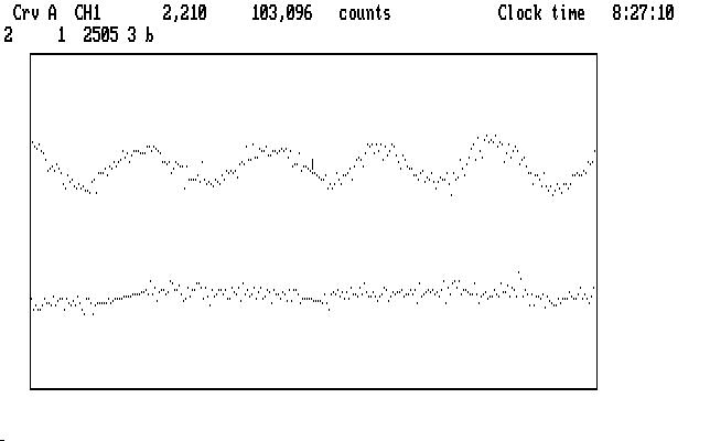
If we smooth both curves shown in Fig. T14 above, using the built-in default smoothing parameter (11), we get this result:

Fig. T15

High frequency measurement noise, caused primarily by atmospheric scintillation, has been significantly reduced in both curves. The bridge in the Ch1 curve fits very comfortably in with the rest of the real data.

Each light curve is accompanied by its own noise, so combining two of them in any way will yield a result that shows more noise than either one alone. Smoothing, where it can be used, minimizes this effect. The most common use is to smooth the sky channel in 3-channel data, prior to subtraction. You can customize your copy of Qed by changing the last line in the qed.ini file with a text editor. Any non-zero value after the smsky entry will invoke automatic sky smoothing in 3-channel runs, and will be used as the smoothing parameter. This action shows up as an oplist entry just before the 'S' or '$' command lines, so replay will do the same thing. By default this action is on, with a parameter of 9, so if you don't want it to happen, you must change the value to 0 in your copy of qed.ini.

While you're right there, you might want to change the autobridging constants, which are 0 by default, meaning autobridging does not occur. If you make them non-zero, the bridging process is invoked (using your supplied values as anchor parameters) just before you write data to disk. This action is dutifully recorded in the oplist as well, just as if you had typed in the command yourself.

Qed only looks at these values on start-up, so if you change them you'll want to re-start the program.